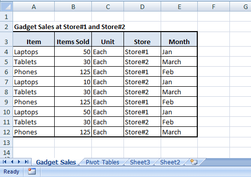
Building A Pivot Table From Multiple Worksheets

Here we will use multiple consolidation ranges as the source of our Pivot Table. You would like to create a pivot table from the data spread across multiple worksheets.

How To Create Two Pivot Tables In Single Worksheet

You can create a PivotTable in Excel using multiple worksheets.

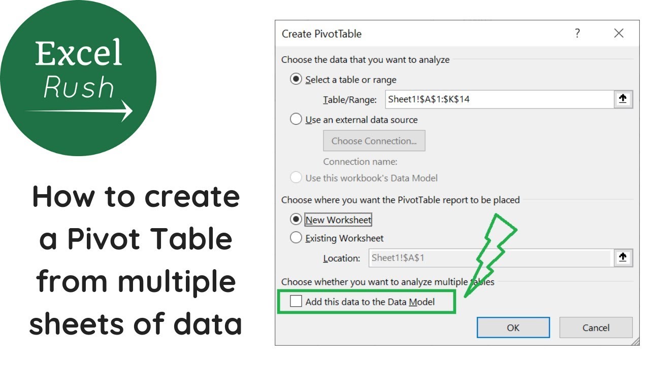
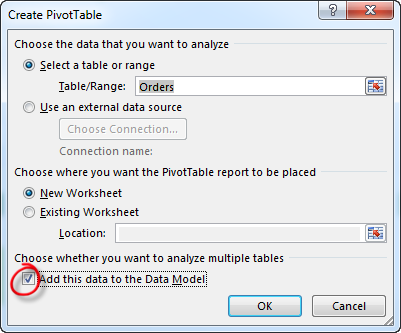
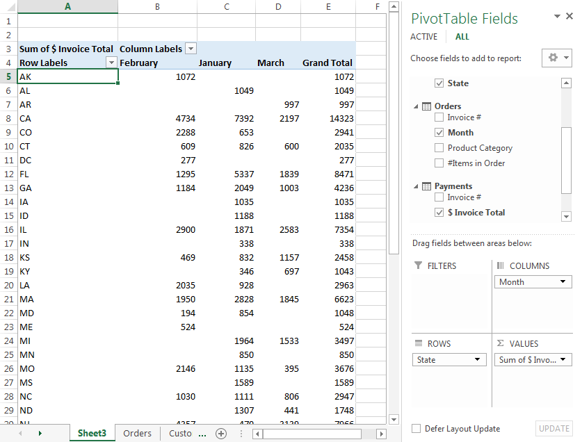
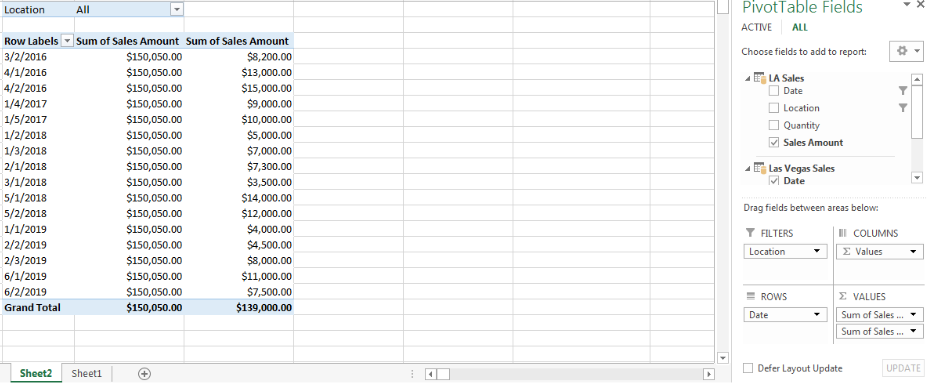
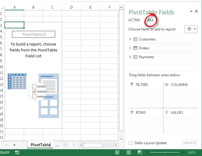
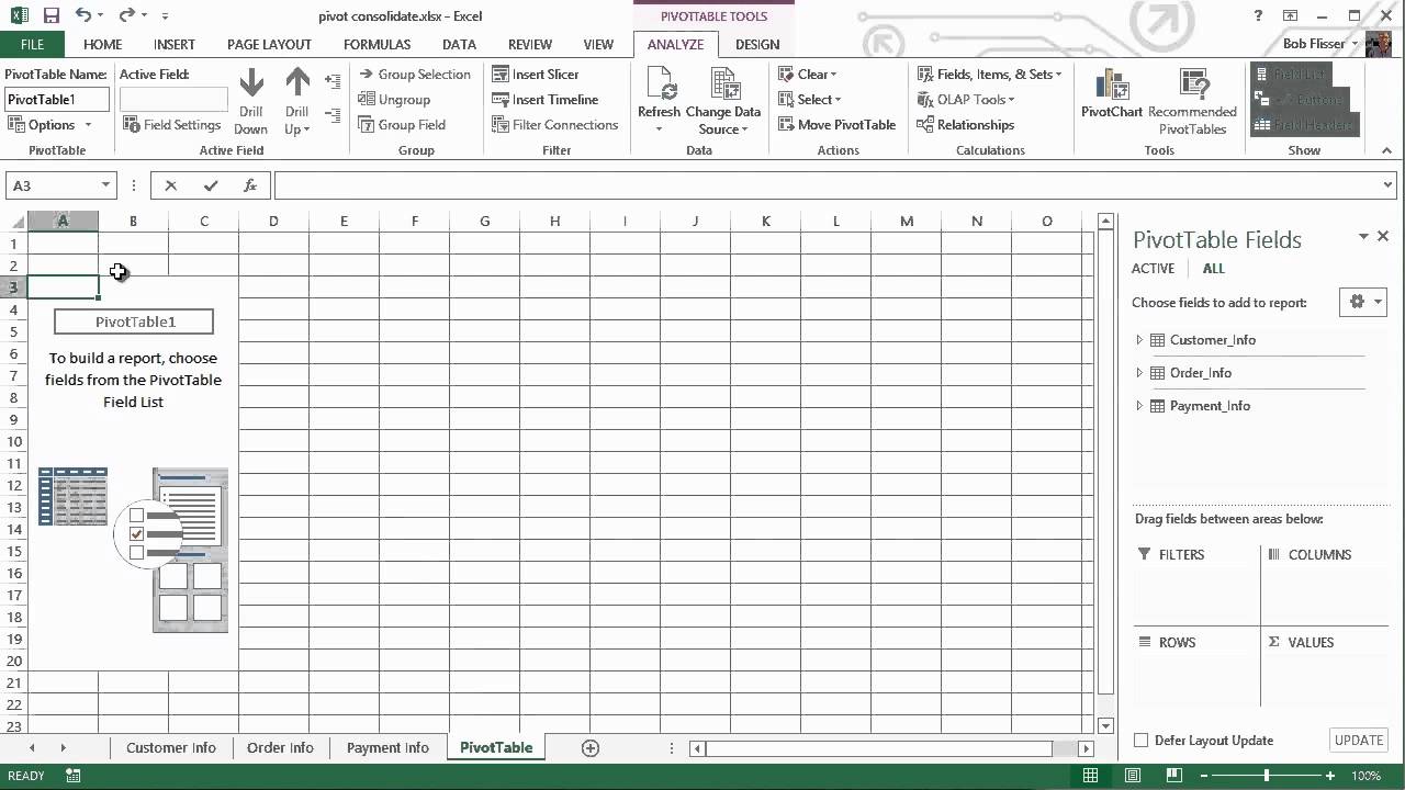
Building a pivot table from multiple worksheets. A Dialog Box will appear now and in that you will be asked whether the Pivot table should be created in a new sheet or the same sheet. Now the table that appears on the screen has the data from all the 4 sheets. From the table on Sheet1 choose Insert Pivot Table and choose the box for Add This Data to the Data Model In the PivotTable Fields pane change from Active to All to reveal all three tables.

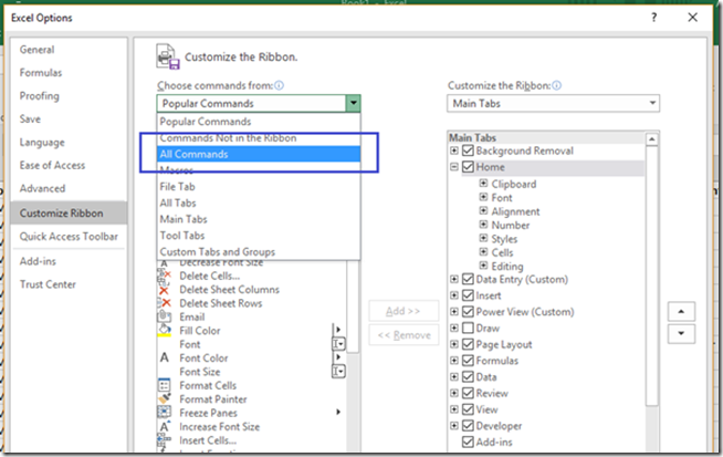
A comprehensive learning site for k-higher 2. Under Choose commands from select All Commands. Click a blank cell that is not part of a PivotTable in the workbook.

A comprehensive learning site for k-higher 2. It is good to use a new sheet. Discover learning games guided lessons and other interactive activities for children.

This is where we are going to Create Pivot Table using Source data from multiple worksheets. The trick to doing this is the tables are related. Create a New Worksheet and name it as Pivot.

5 Press Alt D and then press P. Ad Parents worldwide trust IXL to help their kids reach their academic potential. Ad Parents worldwide trust IXL to help their kids reach their academic potential.

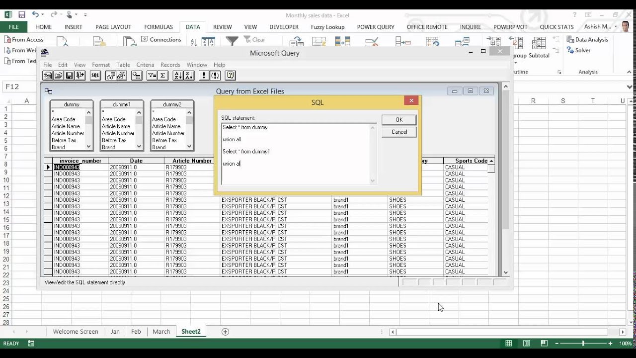
All we need to do is go to File Tab and import that table into Excel. 2 Do the same for the remaining 2 sheets containing the data you want to consolidate. Confirm that the My Table has headers box is checked click OK.

Discover learning games guided lessons and other interactive activities for children. Click on any blank cell in the new Worksheet press and hold ALTD keys and hit the P key twice to fire up the PivotTable Wizard. From the File Menu - click on Return Data to Microsoft Excel.

Ad Download over 30000 K-8 worksheets covering math reading social studies and more. 4 Select a blank cell in the newly created worksheet. On the Tables tab in This Workbook Data Model select Tables in Workbook Data Model.

Youd like to be able to grab similar data from multiple worksheets and summarize it in a pivot table. The Multiple Consolidation feature only works when your data has a single column of text labels on the left with additional numeric columns to the right. Ad Download over 30000 K-8 worksheets covering math reading social studies and more.

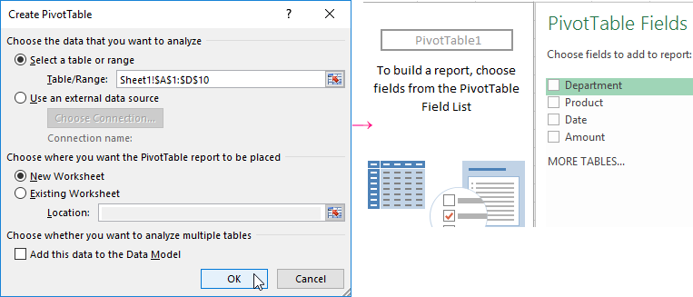
In the Create PivotTable dialog box under Choose the data that you want to analyze click Use an external data source. We can use the Power Table Wizard in Excel to create a pivot table from multiple worksheets. Click Insert PivotTable.

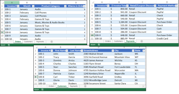
In the list select PivotTable and PivotChart Wizard click Add and then click OK. To create a Pivot Table from the two related tables select Insert tab - Tables group - Pivot Table dropdown arrow - From Data Model. The key is to turn the ranges into Tables.

Begin creating your PivotTable by clicking anywhere in the named table on the first worksheet. Creating a Pivot Table with Multiple Sheets Alt D is the access key for MS Excel and after that by pressing P after that well enter to the Pivot table and Pivot Chart Wizard. The steps below will walk through the process of creating a Pivot Table from Multiple Worksheets.

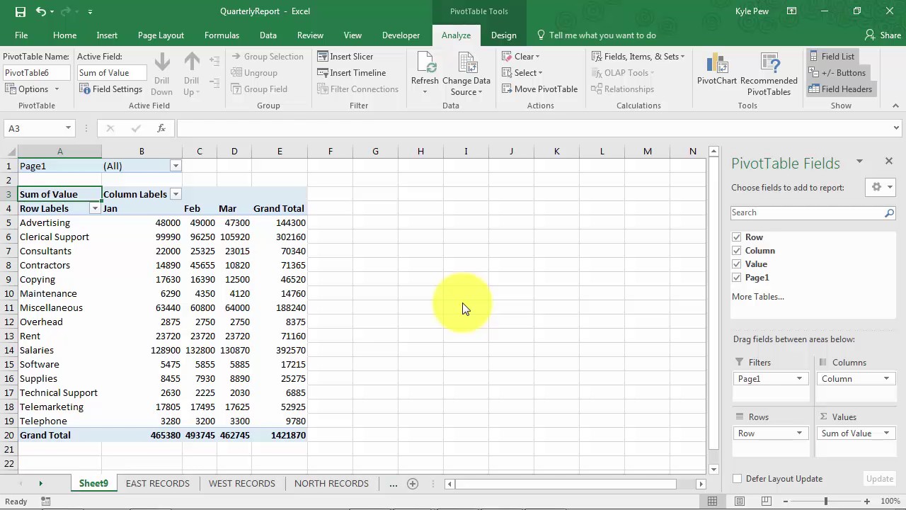
Populate the Pivot Table as needed to answer the applicable business questions. Used by over 10 million students. You can see that in total from all 4 sheets we have 592 records.

Place the Pivot Table on a new sheet. Click on the Insert tab and click on Pivot Tables. 3 It is best to create a new worksheet where this Pivot Table will be located.

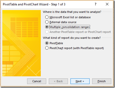
Click any cell on the worksheet. Then click Insert PivotTable to open the Create PivotTable dialog box. On Step 1 page of the wizard click Multiple consolidation ranges and then click Next.

In the end import the data back to excel as a pivot table. Used by over 10 million students. How to Create a Pivot Table from Multiple Worksheets.

As soon as you select fields from more than one table a yellow warning box appears in the PivotTable Fields pane with a button to Create Relationships. Now we can see the Pivot table and Pivot Chart Wizard Step 1 of 3 as shown below. In the example you will click on the Orders table.

How To Create A Pivot Table From Multiple Sheets Of Data Youtube